Tutorial 6: Calibration
Calibration adjusts a model parameter until simulation output matches observed reference data.
This tutorial calibrates x_Temporary_Larval_Habitat — a scale factor that multiplies larval
habitat capacity for all habitat types — to match a reference monthly PfPR curve for
children under 5 (tutorial_6_reference_pfpr.csv).
Interventions are removed for this tutorial so that simulated PfPR reflects baseline transmission only. Tutorial 7 adds interventions back once the right transmission intensity is established.
File: tutorials/tutorial_6_calibration.py
Calibration framework
This tutorial uses idmtools-calibra, which provides four key components:
| Component | Role |
|---|---|
CalibManager |
Orchestrates the calibration loop — runs iterations, collects scores, writes results |
OptimTool |
Gradient-free optimizer: proposes parameter samples each iteration and moves toward better values based on scores |
CalibSite |
Bundles reference data and analyzers for one calibration target |
BaseCalibrationAnalyzer |
Map/reduce framework for scoring simulations against reference data |
CalibManager replaces SimulationBuilder and Experiment from previous tutorials — it
creates and runs experiments internally.
Searching in log space
x_Temporary_Larval_Habitat spans several orders of magnitude (0.0001 to 0.1). Searching
this range in linear space is inefficient because OptimTool's step size is a fixed fraction
of the linear range — steps near 0.1 are proportionally tiny while the same step near 0.0001
overshoots the entire lower region.
The solution is to calibrate in log10 space by defining the parameter as
log10_x_Temporary_Larval_Habitat with bounds [-4, -1]:
OptimTool sees a parameter between -4 and -1 and searches it like any other linear range. Each step of 0.3 log units is a factor of 2× — a consistent proportional step regardless of where in the range the search is. That proportional consistency is why log space explores a parameter spanning orders of magnitude more evenly.
map_sample_to_model_input() converts back to linear space before applying the value to each
simulation:
The linear value is stored as a simulation tag so the analyzer can read it back for plotting.
How OptimTool works
OptimTool is not a random sampler. Each iteration it:
- Fits a linear regression through the previous iteration's samples and scores
- If R² is above the threshold, takes a gradient ascent step — moves the search center in the direction that improves the score
- If R² is below the threshold, jumps to the best-scoring sample
- Draws new samples on a hypersphere around the new center
The search center moves toward the optimum each iteration while the sampling radius stays fixed. You can watch this in the right panel of the plots below — the samples cluster progressively closer to the best value across iterations.
The analyzer: map and reduce
MalariaSummaryAnalyzer subclasses BaseCalibrationAnalyzer and implements two methods:
map(data, item) — called once per simulation. Extracts the last 12 monthly PfPR values
(under-5 age group) from MalariaSummaryReport_monthly.json. The last 12 time steps are the
final year of the 5-year simulation, after the population has reached a stable seasonal
pattern. Age bin index 1 is the 0.25–5 year age group, matching the reference data.
reduce(all_data) — called once per iteration with results from all simulations. Computes
RMSE (Root Mean Square Error) against the reference PfPR, saves a per-iteration CSV, updates
the cumulative plot, and returns scores. Calibra maximizes the score, so reduce() returns
1/RMSE — a closer match produces a higher score.
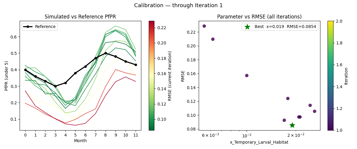
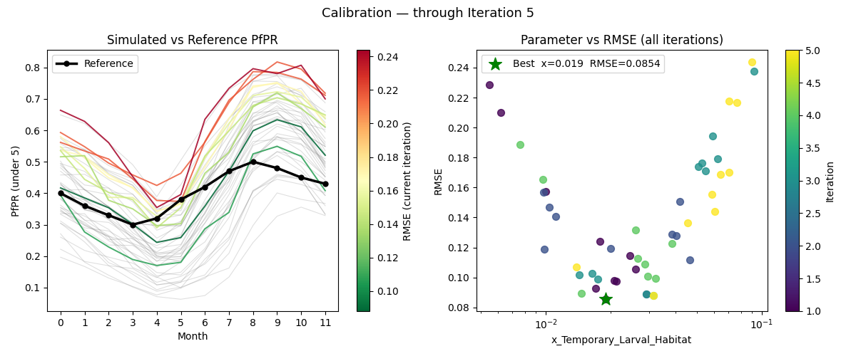
Reading the plots
After each iteration a two-panel plot is saved to tutorial_6_calibration/plots/:
- Left panel — simulated PfPR curves vs the reference (black line). Past iterations are shown in grey; the current iteration is colored green-to-red by RMSE so fit quality is visible at a glance.
- Right panel —
x_Temporary_Larval_Habitatvs RMSE for all iterations, colored by iteration number (dark = early, bright = late). The green star marks the best sample across all iterations.
There is no automated stopping criterion — stop when the fit looks close enough.
Experimenting with the settings
Once the calibration runs, try adjusting these constants and re-running to see how they change the plots.
N_SAMPLES controls how many simulations run per iteration. More samples give OptimTool
more data to fit its linear regression, which means a more accurate gradient estimate and a
better-directed step to the next center. In the right panel you will see more dots per
iteration color. Fewer samples produce a noisier fit — the center may step in the wrong
direction, and you will see more scatter in the right panel. For a single parameter like this
one, 10 samples is usually sufficient. For calibrations with more parameters, a rough guide
is at least 10 samples per parameter.
N_ITERATIONS controls how many times OptimTool moves the center and resamples. More
iterations allow more steps toward the optimum — in the right panel the dots should cluster
progressively closer to the green star as iterations increase, and the grey cloud in the left
panel should thicken while the current iteration's curves get closer to the reference. For
this single-parameter calibration, convergence is usually visible within 3–5 iterations. More
complex calibrations with several parameters need more.
CALIBRATION_PARAMETERS — specifically Guess, Min, and Max:
-
Guessis where OptimTool centers its first hypersphere. A good guess means iteration 1 already explores the right region; a poor guess means the first iteration's PfPR curves in the left panel will all be too high or too low relative to the reference. Try changingGuessfrom-2.0to-3.5or-1.5and watch how iteration 1 looks different. -
MinandMaxdefine the search bounds in log10 space. The green star in the right panel can never fall outside these bounds. If the bounds are too narrow and exclude the true value, the calibration will converge to the boundary. If they are too wide, more iterations are needed to explore the space. The current bounds[-4, -1]correspond to[0.0001, 0.1]in linear space — a range that covers several orders of magnitude and is wide enough for most single-site malaria calibrations.
Using the calibrated value in Tutorial 7
When calibration finishes the script prints the best-fit log10 value to the terminal:
============================================================
NEXT STEP: open tutorial_6_calibration/CalibManager.json, find
  final_samples -> log10_x_Temporary_Larval_Habitat[0]
  and paste that value into CALIBRATED_LOG10_X_LARVAL_HABITAT
  in tutorial_7_burnin.py and tutorial_7_pickup.py
============================================================
Open tutorial_6_calibration/CalibManager.json and look for:
If final_samples is not in CalibManager.json
This key is only written when all iterations complete. If calibration was stopped early,
look at the right panel of the iteration plots — the green star marks the best sample
across all completed iterations. Use that x_Temporary_Larval_Habitat value, converting
it to log10 space (log10(value)), or pick the best row from any
tutorial_6_calibration/iter*/pfpr_records.csv by choosing the row with the lowest RMSE.
Paste the value into both tutorial_7_burnin.py and tutorial_7_pickup.py —
CALIBRATED_LOG10_X_LARVAL_HABITAT must be the same in both scripts:
Both scripts convert the log10 value to linear space automatically (10 ** value) —
you do not need to do the conversion yourself.
Calibration progress
Iteration 1
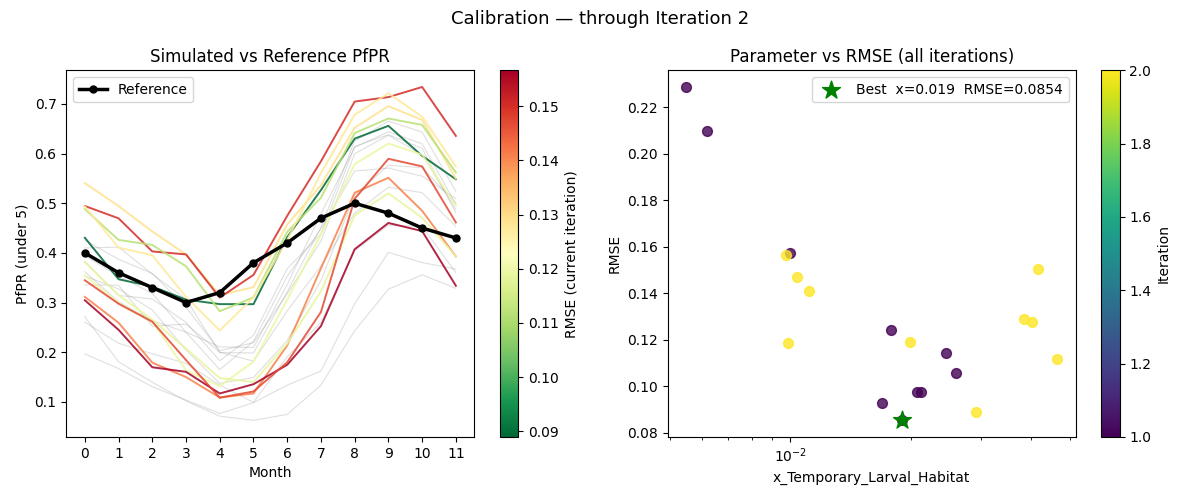
Iteration 2
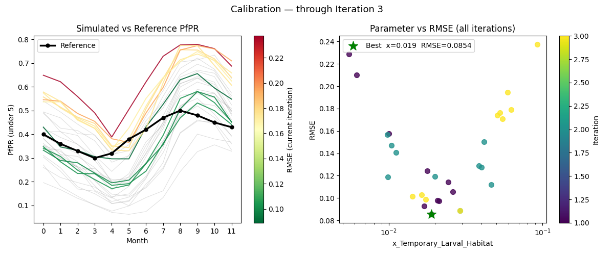
Iteration 3
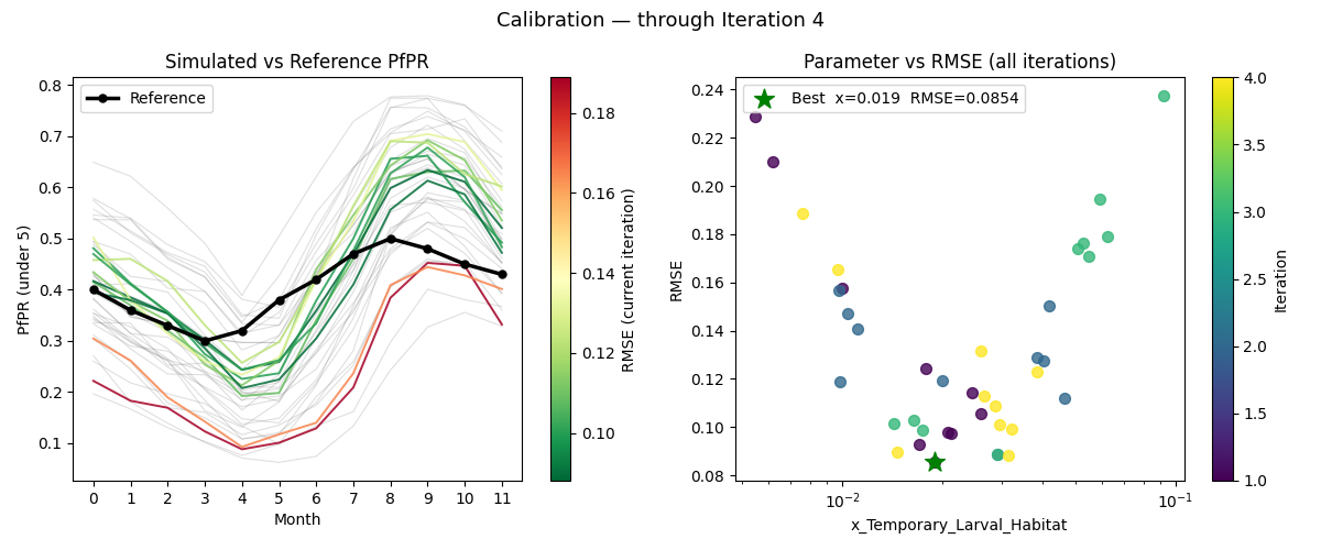
Iteration 4
Iteration 5
Iteration 15
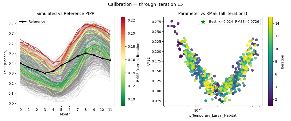
With N_SAMPLES=40 and N_ITERATIONS=15, the curves in the left panel have converged tightly around the reference line, and the right panel shows the parameter-vs-RMSE scatter clustered near the green star. Compare this to iteration 1, where the curves were spread across a wide range. More samples and iterations allow OptimTool to take more confident steps and narrow in on the best value.
Next
Tutorial 7 uses the calibrated value to run a burnin to equilibrium, then starts intervention scenarios from the serialized population.